Listen to this Post
Introduction:
In the high-stakes world of RF engineering, the difference between a system that jams an enemy drone and one that blinds your own radar often comes down to a few turns of a tuning screw. Cavity filters are the unsung heroes of the RF front-end, serving as the gatekeepers that allow only the desired signals to pass while ruthlessly rejecting out-of-band interference and noise. However, while the hardware is inherently analog, the skills required to tune a 5-resonator cavity for a 100 MHz bandwidth at 2.4 GHz have become a critical technical intersection, blending the physics of electromagnetic resonance with the precise data offered by a modern Vector Network Analyzer (VNA). For professionals in C-UAS (Counter-Unmanned Aerial Systems), telecom, and defense, mastering this is a non-1egotiable requirement for system survivability and performance.
Learning Objectives:
- Understand the relationship between mechanical screw adjustments (6-32 and 4-40) and their effects on S-parameters.
- Learn the iterative, sequential process for tuning a cavity filter to achieve <1.0 dB insertion loss and >20 dB return loss.
- Leverage VNA data to mathematically transform physical adjustments into a passband with minimal ripple and maximum power transfer.
You Should Know:
- The VNA and the Math Behind the Filter Curve
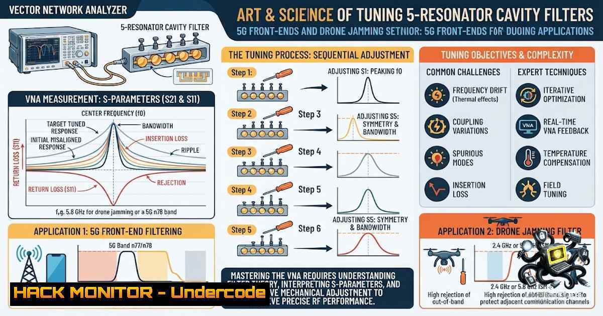
The Vector Network Analyzer is the “truth machine” for this process. It sweeps frequency across the desired range (2.35 to 2.45 GHz) and measures the incident, reflected, and transmitted waves through the device under test. When tuning, you are controlling two critical parameters.
– Insertion Loss (S21): This is the measure of forward gain or loss. Mathematically, S21 (dB) = -10 log10(Pout / Pin). A reading of 0 dB would mean all power is transferred; we aim for less than 1.0 dB loss.
– Return Loss (S11): This measures impedance matching. It is defined as S11 (dB) = -10 log10(|Γ|²), where `Γ` (Gamma) is the voltage reflection coefficient. A target of >20 dB return loss implies a VSWR (Voltage Standing Wave Ratio) of approximately 1.22:1, meaning only ~1% of the incident power is reflected back to the source.
Before starting, ensure the VNA is calibrated using a SOLT (Short-Open-Load-Thru) calibration kit at the 2.4 GHz frequency range. This eliminates the systematic errors introduced by test cables and adapters.
- Understanding Your Tools: The 6-32 and 4-40 Screws
The cavity filter is a physical manifestation of lumped LC circuits. You don’t have capacitors and inductors in the traditional sense; the resonator rods act as inductors, and the gap between the rod and the cavity wall acts as the capacitor.
– The 6-32 Screws (Frequency Adjust): These are the large screws protruding into the center of the resonator. Think of them as variable capacitors. When you screw them deeper into the cavity, you increase the capacitance between the rod and the wall. As Fc = 1 / (2 π √(Leq Ceq)), increasing C lowers the frequency. Conversely, backing them out raises the center frequency of that specific cavity.
– The 4-40 Screws (Coupling/Bandwidth Adjust): Located on the irises between cavities, these control the magnetic or electric coupling. By screwing the 4-40 screw further into the window, you increase the coupling coefficient. This usually widens the overall bandwidth but risks introducing ripple (an uneven passband). It’s a delicate trade-off.
3. Step-by-Step Tuning Procedure: The Sequential Approach
Tuning is an iterative process, but a specific sequence ensures convergence.
1. Connect and Observe: Connect the filter to the VNA ports via SMA cables. Set the VNA to display both S11 and S21 on a split screen.
2. Initial Sweep: Perform a wide sweep from 2.3 GHz to 2.5 GHz. You should see a ripple or a single resonance dip.
3. Frequency Alignment: Starting at Cavity 1 (input), adjust its 6-32 screw. Watch the S21 trace. Screw in to lower the dip frequency, or out to raise it. A quarter-turn often shifts several megahertz.
4. Shape the Bandwidth: With the input and output aligned, adjust the 4-40 coupling screws between Cavity 1-2 and Cavity 4-5. If the bandwidth is narrower than 100 MHz, turn these screws in to increase coupling.
5. Tune the Center Resonators: The center cavities (3 and 4) have the most profound impact on return loss. Use these 6-32 screws to “flatten” the top of the passband and “dip” the S11 curve to -20 dB.
6. Iterate: Every time you change a coupling screw (4-40), the center frequency of the adjacent resonators shifts. Re-adjust the 6-32 screws slightly. This process requires 5–10 passes.
4. Linux Terminal Commands for VNA Automation (SCPI)
For those using a programmable VNA connected to a Linux or macOS machine, automation scripts save time. Python is the go-to language for integrating with SCPI (Standard Commands for Programmable Instruments).
import pyvisa
import time

rm = pyvisa.ResourceManager()
vna = rm.open_resource('TCPIP0::192.168.1.2::inst0::INSTR')  VNA IP address

Reset and configure the VNA
vna.write('RST; CLS')
vna.write('SENS1:SWE:POIN 1001')  Set 1001 sweep points
vna.write('SENS1:FREQ:STAR 2.35E9; STOP 2.45E9')
vna.write('CALC1:PAR:EXT S21')  Measure S21

Trigger a sweep and fetch the maximum ripple
data = vna.query('CALC1:DATA? SDATA')
print(data)
On Windows, using the Keysight Connection Expert or similar software allows you to execute similar scripts via PowerShell or MATLAB, leveraging `visa` libraries.
- Windows Power Commands for Network Capture (Security Context)
While tuning the hardware is key, monitoring the “air” is just as important. While this isn’t directly a software filter, in C-UAS applications, ensuring your filter is rejecting 2.45 GHz WiFi interference often means using spectrum analyzers in tandem. If you are using a Software Defined Radio (SDR) hooked to the filtered output, Windows systems can utilize these commands to view live waterfall graphs.If using an SDR (e.g., RTL-SDR) you typically don't use native Windows cmdlets but third-party software like SDR. However, for analyzing the RF environment via a network analyzer or SDR, you can use WSL (Windows Subsystem for Linux). wsl --install Install GQRX or rtl-sdr tools inside WSL. sudo apt update && sudo apt install rtl-sdr gqrx-sdr
In a hardened environment (API security in telecom), ensuring that your RF front-ends aren’t exposing vulnerabilities often involves checking the SNMP (Simple Network Management Protocol) data of the tower equipment. Use `netstat -an | findstr “161”` to see if the management interface is listening on the expected ports.
-
The “Golden Rule” of Return Loss and Ripple
Your primary enemy in tuning is Ripple. A perfectly flat passband is the goal.
– If you over-couple (4-40 screws too deep), you get an S21 curve that looks like a “dip” in the middle (bad).
– If you under-couple, you get a sharp peak in the center.
– The fix: Adjust the 6-32 screws of the input and output resonators slightly outward to “pull” the S21 trace up, while pushing the coupling screws back one flat-head turn to reduce the ripple.
The math governing this is the Chebyshev or Butterworth polynomial response. For a 5-pole Chebyshev design with 0.1 dB ripple, the group delay is inherently nonlinear, but a skilled tuner minimizes this by adjusting the 4-40 screws until the S11 dips are equal in magnitude across the entire frequency span.
7. Practical Tuning Tips for the Bench
- Use a Torque Wrench: SMA connectors are rated for 8 in-lbs. Overtightening can deform the connector pin, changing the impedance and ruining your return loss target.
- The Marker Method: Set VNA markers at 2.35 GHz, 2.4 GHz, and 2.45 GHz. Tune so that S11 at 2.4 GHz is below -20 dB and S21 at the edges is only 3 dB down (the standard 3 dB bandwidth).
- Temperature Sensitivity: Cavity filters drift with temperature. Use a thermal chamber if the filter will be used outdoors in extreme conditions (like on a drone jammer). Re-tune it at the operating temperature.
What Undercode Say:
- Key Takeaway 1: The abstract math of LC circuits becomes physical reality via 6-32 and 4-40 screws; recognizing that tuning the center resonator is the secret to achieving the desired return loss.
- Key Takeaway 2: The interplay between bandwidth and ripple is a zero-sum game; you cannot widen the bandwidth without sacrificing insertion loss, and only the VNA reveals the true balance.
Analysis:
This hands-on skill highlights a critical gap in modern IT and cybersecurity education: most offensive and defensive cyber operators understand the bits and bytes but are wholly detached from the physical layer. A drone jamming system that is poorly tuned not only fails to defeat the target UAV but might also cause self-interference, effectively jamming the operator’s own command link. This is a vulnerability at the hardware layer that no firewall or zero-day exploit can fix. Furthermore, as we move towards 5G and 6G Open RAN architectures, the interoperability of these passive components becomes vital. The ability to generate, capture, and interpret S-parameter data is becoming a non-1egotiable skill for RF verification engineers, bridging the gap between software-defined networking and classical high-frequency engineering. The “art” mentioned is essentially recognizing the correct sequence and depth of adjustments, which only experience teaches.
Prediction:
- -1 Automation is taking over: While currently a human-centric art, the increasing availability of cheap, vector network analyzers and AI-driven algorithms will lead to automated “robot tuners” that can trim these screws faster than a human, reducing the demand for entry-level RF bench tuners.
- +1 The Criticality of 2.4 GHz: With the proliferation of commercial drones and IoT devices, the ability to selectively filter and jam or protect the 2.4 GHz band will make RF engineers the new security gatekeepers, especially in critical infrastructure (airports, power plants).
- +1 Resurgence of Hardware Skills: As cybersecurity moves to the physical layer (e.g., RF jamming, side-channel attacks), we will see a resurgence of demand for hybrid professionals who understand S-parameters, Python automation, and spectrum security.
▶️ Related Video (72% Match):
🎯Let’s Practice For Free:
🎓 Live Courses & Certifications:
Join Undercode Academy for Verified Certifications
🚀 Request a Custom Project:
Secure, high-velocity infrastructure and disruptive technological engineering. Contact our engineering team for high-tier development and proprietary systems:
[email protected]
💎 Smart Architecture | 🛡️ Secure by Design | ⭐ Trusted by Thousands
IT/Security Reporter URL:
Reported By: Itsik Za – Hackers Feeds
Extra Hub: Undercode MoN
Basic Verification: Pass ✅


